Uncertainty Intervals are better than p-values. Sure, its better to use both, but p-values are just a point estimate and they bring no concept of uncertainty in our estimate - this can lead to situations where we expose ourselves to high downside risk.

Take the following example for instance. Let’s say we’re running a “Do no harm” A/B test where we want to roll out an experiment as long as it doesnt harm conversion rate.

If you want to follow along with the code, see here.

The experiment design

Given the stakeholders want to rule out a drop in conversion, and ruling out small differences requires large sample sizes, we decide to design an experiment with good power to detect the presence of a 0.5% absolute drop (if one were to truly exist)

We ran a power analysis and found that in order to have a 90% probability of detecting (power=0.9) a 0.5% absolute drop in conversion rate with 80 percent confidence ( 𝛼=0.2 ), we need N=32500 per group

Statisticians might not love this interpretation of a power analysis, but its a useful and interpretable translation and tends to coincide with what we’re aiming for anyway. In reality, frequentist power analyses assume that the null hypothesis is correct, which isn’t quite what we want, not to mention, frequentist power analyses use backwards probabilities which are just plain confusing - see here to for more

Note that we’re prioritizing power here for a reason. If 𝛼 is false positive rate, and power is probability of detection, then don’t we want to prioritize our probability of detecting a drop if one truly exists? A false negative here would be more expensive then a false positive

Running the code below leads us to conclude are sample size should be roughly 32,500 users per group.

import statsmodels.api as sm
import numpy as np
import pandas as pd
import seaborn as sns
import matplotlib.pyplot as plt
import matplotlib.ticker as mtick
from IPython.display import display, Math, Latex


pA = 0.1 # historical conversion rate
abs_delta = 0.005 # minimum detectable effect to test for

# Statsmodels requires an effect size 
# (aka an effect normalized by its standard deviation)
stdev = np.sqrt( pA*(1-pA) ) # bernoulli stdev, sigma = sqrt(p(1-p))
ES = abs_delta / stdev 

# estimate required sample size
sample_size = sm.stats.tt_ind_solve_power(
    -ES, 
    alpha=0.2,
    power=0.9,
    alternative="smaller"
)
int(sample_size)

The experiment

I’m going to simulate fake data for this experiment where

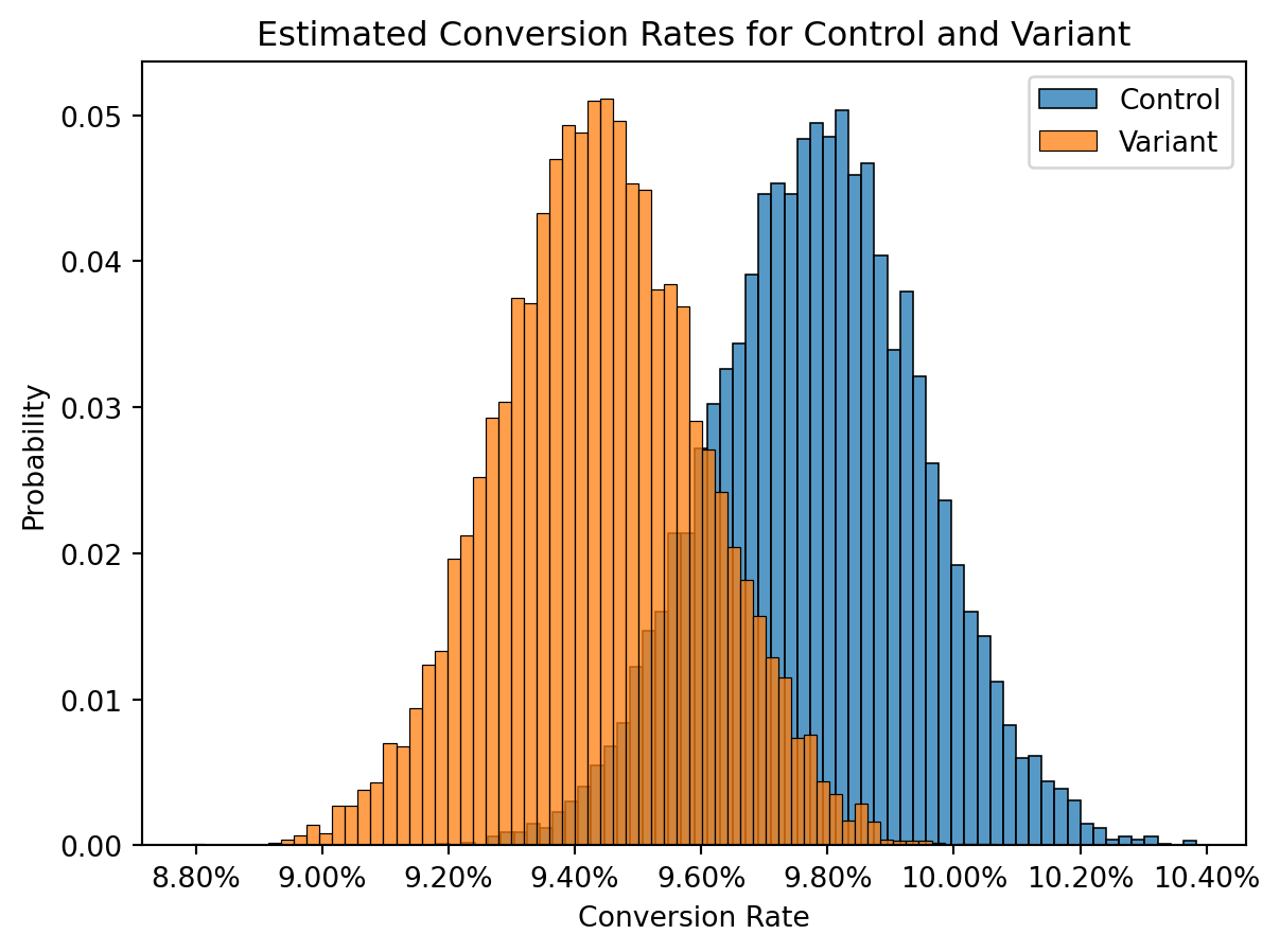
The control has a true conversion rate of 10%
the variant has a true conversion rate of 9.25%

For examples sake we’ll pretend we don’t know that the variant is worse

Code

# Settings
SEED = 14
np.random.seed(SEED)
N = 32500
pA = 0.1
pB = 0.0925

# Simulation
def simulate_experiment(pA, pB, N_per_group):
    
    df = pd.DataFrame({
        "group":["A"]*N + ["B"]*N,
        "convert":np.r_[
             np.random.binomial(1, p=pA, size=N),
             np.random.binomial(1, p=pB, size=N)
        ]
    })
    
    return df

df = simulate_experiment(pA, pB, N)

def summarize_experiment(df):
    return (
        df.groupby("group")
        .convert.agg(['mean', 'sum', 'count'])
        .set_axis(['Conversion Rate', 'Conversions', 'Sample Size'], axis=1)
    )

df.pipe(summarize_experiment).style.format({"Conversion Rate": "{:.2%}"})

	Conversion Rate	Conversions	Sample Size
group
A	9.78%	3179	32500
B	9.43%	3066	32500

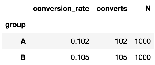
Looking at the data above, we’re seeing a slightly worse conversion rate in the variant, but barely. We run a two-proportions z-test and we find that there’s a non-significant p-value, meaning we found insufficient evidence of the variant having lower conversion than the control.

def pval_from_summary(tab):
    
    _, pval = sm.stats.proportions_ztest(
        count=tab["Conversions"], 
        nobs=tab["Sample Size"],
        alternative="two-sided"
    )
    return pval

pval = (df.pipe(summarize_experiment)
   .pipe(pval_from_summary))
display(Math(rf"p = {round(pval, 3)}"))

\(\displaystyle p = 0.133\)

We recommend to our stakeholders to roll out the variant since it “does no harm”

There are some serious red flags here

First of all, p-values are all about the null hypothesis. So just because we don’t find a significant drop in conversion rate, that doesnt mean one doesnt exist. It just means we didnt find evidence for it in this test
Second, there was no visualization of the uncertainty in the result

Understanding Uncertainty with the Beta Distribution

For binary outcomes, the beta distribution is highly effective for understanding uncertainty.

It has 2 parameters

alpha, the number of successes
beta, the number of failures

It’s output is easy to interpret: Its a distribution of plausible probabilities that lead to the outcome.

So we can simply count our successes and failures from out observed data, plug it into a beta distribution to simulate outcomes, and visualize it as a density plot to understand uncertainty

Code

np.random.seed(SEED)
samples = 10000

A = df.query("group=='A'").convert.values
B = df.query("group=='B'").convert.values

# sample uncertainty
pA = np.random.beta(A.sum()+1, len(A)-A.sum()+1, size=samples)
pB = np.random.beta(B.sum()+1, len(B)- B.sum()+1, size=samples)

# Plot
fig, ax = plt.subplots()
sns.histplot(pA, label='Control', stat='probability',ax=ax)
sns.histplot(pB, label='Variant', stat='probability',ax=ax)
ax.legend()
ax.set_title("Estimated Conversion Rates for Control and Variant")
ax.set_xlabel("Conversion Rate")
ax.xaxis.set_major_formatter(mtick.PercentFormatter(1,2))

plt.show()

It’s also easy to work with - if we want to understand the plausible differences between groups, we can just take the differences in our estimates

\[ \delta = \hat{p_B} - \hat{p_A} \]

Code

np.random.seed(SEED)
samples = 10000

fig, ax = plt.subplots()
sns.histplot(pB - pA, label='Control', stat='probability',ax=ax)
ax.legend()
ax.set(
    title="Avg Treatment Effect Estimate",
    xlabel="Avg Treatment Effect (Absolute)"
)
ax.axvline(0, ls='--', color='k')
ax.xaxis.set_major_formatter(mtick.PercentFormatter(1,2))
plt.show()

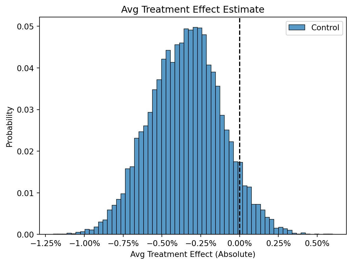
With visualization, we get a very different picture than our non-significant p-value. We see that there’s plenty of plausibility that the control could be worse.

We can further calculate the probability of a drop greater than 0.5%, \(P(\delta \: < -0.5\%)\)

# P(B - A < -0.5%) 
contrast = (pB - pA)
prob = (contrast < -0.005).mean()
display(Math(f"P(\delta \: < -0.5\%) = {prob*100:.1f}\%"))

\(\displaystyle P(\delta \: < -0.5\%) = 25.5\%\)

Remember when we designed the experiment? Considering our main goal was to do no harm, we might not feel so confident in that now, and rightly so, we know the variants worse since we simulated it.

Unless the expected cost of this change isn’t that high in one of the worst case scenarios of that uncertainty interval, we shouldnt feel very confident in rolling out this variant without further consideration.

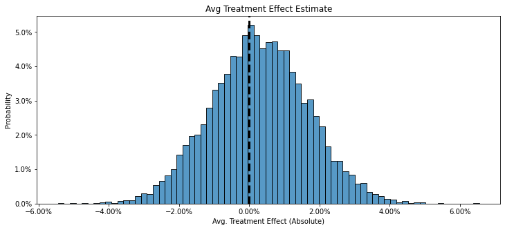
This is particularly important with higher uncertainty. We can see this more clearly in another example below where the observed conversion rate is better in the variant, but the downside risk is as high as a 4% drop in conversion rate.

\[ p = 0.59 \]

Another Example: Which Metric?

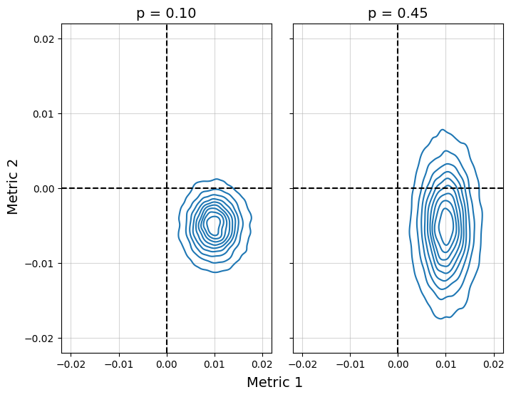
This is a fun problem from @seanjtaylor > “You run a product test and measure a strong positive effect on your first metric.

Metric 1: +1% (p<.01)

You also see a negative, but not significant result on equally important Metric 2. You only care about these two metrics. Which of these estimates would you prefer to ship?”

Metric 2: -0.5% (p = 0.10)

Metric 2: -0.5% (p=0.45)

Neither is shippable

Try to think it through on your own first, then scroll down for the answer

If you chose option 2, you weren’t alone. Option 1 makes it seem like there’s a more likely negative effect due to the lower p-value, so thats worse, right?

Not quite. Check out the uncertainties. The downside risk option 2 is much worse than option 1.

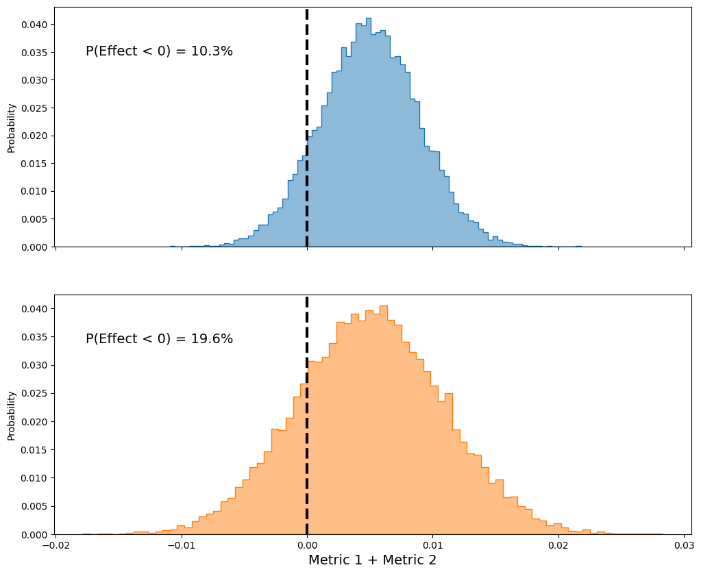
We can take this one step further and add our effects to compare (remember we assumed the metrics are equally important), and see if it’s overall net positive

As shown above, the non significant p value option has a higher probability of being negative, AND it gives more plausibility to more negative possible effects

Summary

Always report uncertainty intervals - p-values definitely dont tell the whole story, even with well designed experiments. As we saw, ignoring uncertainty can expose ourselves to high downside, especially when our choice in experiment design has even the slightest bit of arbitrary choices involved (such as an arbitrary minimum detectable effecs)

Reporting uncertainty intervals or beta distributions (or even bootstrapping) can be a great way to avoid falling for this mistake