I recently saw a viral linkedin post discussing how multicollinearity will ruin your regression estimates. The solution? Simply throw out variables with high Variance Inflation Factors and re-run your regression.
Let me tell you, don’t do this. A fear of multicollinearity is this misconception in data science that is far too prevalent.
I’ve seen the same assumptions with correlation - if two variables are very highly correlated people assume they shouldn’t be in the same model. I’m going to show you why 1) these approaches are a mistake and 2) you can’t escape domain knowledge when informing your regression.
A simulation
We’re going to simulate a fake scenario. You want to know the effect of some variable \(X_3\) on \(y\) with your regression. The data generating process is below
The simulation below makes it clear the true effect of \(X_3\) on \(y\) is 0.7, so we know our regression should hopefully return it as an estimate
Code
import numpy as np
import pandas as pd
import statsmodels.api as sm
from statsmodels.stats.outliers_influence import variance_inflation_factor as vif
import matplotlib.pyplot as plt

N = 250
SIG = 0.5
TRUE_EFFECT = 0.7

rng = np.random.default_rng(99)
df = (
    pd.DataFrame({
    "x1":rng.normal(0, 1, size=N),
    "x2":rng.normal(0, 1, size=N)}
    )
    # simulate x3 as a function of x1
    .assign(x3=lambda d: rng.normal(1.1 + d.x1*3.8, SIG))
    # simulate y as a function of x1,x2,x3
    .assign(y = lambda d: rng.normal(0.5 + d.x1*-4 + d.x2*-0.5 + d.x3*TRUE_EFFECT, SIG))
)
df.head().round(2)| x1 | x2 | x3 | y | |
|---|---|---|---|---|
| 0 | 0.08 | 0.54 | 1.96 | 1.94 |
| 1 | -0.46 | 1.59 | 0.08 | 1.33 |
| 2 | 0.05 | -0.69 | 0.81 | 1.01 |
| 3 | 0.69 | 0.47 | 3.44 | 0.53 |
| 4 | -1.76 | -0.77 | -5.98 | 3.36 |
Lets take a look at the variance inflation factors below
Code
X = df.filter(like='x')
pd.DataFrame(
    {"VIF": [vif(X.values, i) for i in range(X.shape[1])]},
    index=X.columns
).round(2)| VIF | |
|---|---|
| x1 | 10.35 |
| x2 | 1.00 |
| x3 | 10.35 |
Based on this, we supposedly should remove \(X_1\) from our regression (VIFs of 5-10 are considered high).
If we look at the correlation, we reach the same conclusions - \(X_1\) has high correlation with \(X_3\) so supposedly “they provide the same information and only 1 is useful”
X.corr().loc['x3']x1 0.990898
x2 -0.020267
x3 1.000000
Name: x3, dtype: float64Does it work?
We’re going to fit two regressions - one that follows the advice of throwing out variables with high VIFs or correlation - and another that is informed by domain knowledge.
# vif/correlation informed variable selection
m1 = sm.OLS.from_formula("y ~ x2 + x3", data=df).fit()

# domain knowledge informed variable selection
m2 = sm.OLS.from_formula("y ~ x1 + x2 + x3", data=df).fit()
Code
def plot_ci(model, ax, color='C0', label=None):
    lb = (model.params - model.bse*2)
    ub = model.params + model.bse*2
    ax.hlines(0, lb.loc['x3'], ub.loc['x3'], lw=2, label=label, color=color)
    ax.scatter(model.params.loc['x3'], 0, facecolor='white', edgecolor=color, zorder=10, s=10)


fig, ax = plt.subplots()
plot_ci(m1, ax=ax, color='C1', label='VIF/Corr. informed model')
plot_ci(m2, ax=ax, color='C0', label='Causally informed model')

ax.axvline(0, ls='--', color='k')
ax.axvline(TRUE_EFFECT, color='r', ls='--', lw=1, label='True Effect')
ax.set_xlim(-1,1)
ax.set_ylim(-1,1)
ax.set_yticks([])
ax.set(title="Estimated effect of X3 -> y", xlabel="Beta Coefficient")
ax.legend()
plt.show()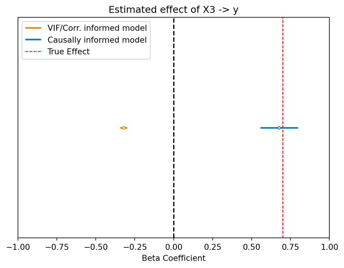
Not only is the VIF informed model wrong, but more importantly it actually thinks \(X_3\) has a negative effect instead of a positive effect!
Why did this happen?
Lets go back to our data generating process
It’s clear that \(X_1\) causally effects both \(X_3\) and \(y\) - this makes it a confounding variable, or a “backdoor” for \(X_3\). If we want our regression to have proper estimates of \(X_3\), we therefore need to make sure our regression model accounts for \(X_1\) to de-bias \(X_3\).
A classic (and dark) example is the ice-cream and drowning relationship. As people eat more ice cream there tend to be more drownings. Why? Warm weather causes ice cream and increased pool and beach use lead to the unfortunate increase in drownings. Accounting for warm weather explains away this relationship, and thats exactly how regression can work.
This is why its so important to incorporate domain knowledge in your modeling. Mapping pout the data generating process and using it to inform your model is always the right choice. For more on this check out A Crash Course on Good and Bad Controls. I also really like Richard McElreath’s discussion on this in his 2nd edition of Statistical Rethinking.